T-SIM V4.5 Reference
T-SIMFIT Version 1.4 Manual
Stress-strain data at three strain rates and three temperatures are required. It is possible to make measurement at one temperature with three strain rates. At the remaining two temperatures it is possible to measure just at one strain rate.
There are four possible types of the measured stress-strain curves which can be used in T-SIMFIT:
The preferred type is the last one - Equibiaxial extension data with exponential extension ratio - time dependency.
Detailed description of the possible types of tests
The tested specimen is deformed in just one direction, the remaining two directions are free:
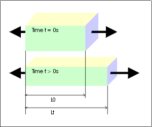
L0 is an initial sample length.
Lt is a sample length at time t.
l1(t) is an extension ratio in the direction
of elongation, defined as
l1(t) = Lt / L0.
Moreover, l1 is a linear function of time in this case:
l1(t) = Lt / L0 = L0(1 + at) / L0 = 1 + at, where
a is a constant corresponding the speed of deformation (a is equal to the speed in mm/s divided by initial sample length).
The extension ratii in the two remaining directions are defined as
l2l3 = 1 / l1 = 1 / (1 + at),
and
l2 = l3.
As the sample deforms, the corresponding force F generated in the material is measured. Using the measured forces F(t) and recorded l1(t), the stress s(l1(t)) at extension ratio l1(t) is calculated:
s(l1(t)) = F(t) / A(t) = F(t) / ( A0 / (1 + at)), where
A0 is the initial sample cross-section area,
A(t) is the sample cross-section area at time t.
The calculated values of s for different values of l have to be input into T-SIMFIT. It means that only true stresses and true extension ratii can be used ! Do not use engineering stresses or engineering extension ratii !
2. Uniaxial elongation data with exponential extension ratio - time dependency:
The geometrical situation is the same as in the case 1. The difference is in the extension ratio - time dependency. Now, l1 is an exponential function of time:
l1(t) = Lt / L0 = L0exp(et) / L0 = exp(et), where
e is the strain rate in 1/s.
The extension ratii in the two remaining directions are defined as
l2l3 = 1 / l1 = 1 / exp(et) ,
and l2 = l3.
As the sample deforms, the corresponding force F generated in the material is measured. Using the measured forces F(t) and recorded l1(t), the stress s(l1(t)) at extension ratio l1(t) is calculated:
s(l1(t)) = F(t) / A(t) = F(t) / ( A0 / exp(et)), where
A0 is the initial sample cross-section area,
A(t) is the sample cross-section area at time t.
The calculated values of s for different values of l have to be input into T-SIMFIT. It means that only true stresses and true extension ratii can be used ! Do not use engineering stresses or engineering extension ratii.
3. Biaxial extension data with linear extension ratio - time dependency:
The tested specimen is deformed in two directions, the remaining one direction is free.
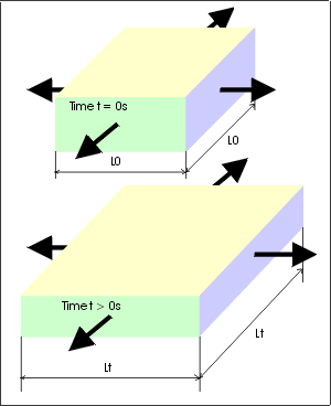
L0 is an initial sample length.
Lt is a sample length at time t
l1(t) = l2(t)
is an extension ratio in the directions of extension, defined as
l1(t) = l2(t) = Lt / L0.
Moreover, l1 and l2 is a linear function of time in this case:
l1(t) = l2(t) = Lt / L0 = L0(1 + at) / L0 = 1 + at, where
a is a constant corresponding the speed of deformation (a is equal to the speed in mm/s divided by initial sample length).
The extension ratio in the one remaining direction is defined as
l3 = 1 / (l1l2) = 1 / (1 + at)^2.
As the sample deforms, the corresponding force F generated in the material is measured. Using the measured forces F(t) and recorded l1(t) (equal to l2(t)), the stress s(l1(t)) at extension ratio l1(t) is calculated (the same equation is valid for l2(t)):
s(l1(t)) = F(t) / A(t) = F(t) / ( A0 / (1 + at)), where
A0 is the initial sample cross-section area,
A(t) is the sample cross-section area at time t.
The calculated values of s for different values of l have to be input into T-SIMFIT. It means that only true stresses and true extension ratii can be used ! Do not use engineering stresses or engineering extension ratii.
4. Biaxial extension data with linear extension ratio - time dependency:
The geometrical situation is the same as in the case 3. The difference is in the extension ratio - time dependency. Now, l1 and l2 are exponential functions of time:
l1(t) = l2(t) = Lt / L0 = L0exp(et) / L0 = exp(et), where e is the strain rate in 1/s. The extension ratio in the one remaining direction is defined as
l3 = 1 / (l1l2) = 1 / (exp(et))^2 .
As the sample deforms, the corresponding force F generated in the material is measured. Using the measured forces F(t) and recorded l1(t) (equal to l2(t)), the stress s(l1(t)) at extension ratio l1(t) is calculated (the same equation is valid for l2(t)):
s(l1(t)) = F(t) / A(t) = F(t) / ( A0 / exp(et)), where
A0 is the initial sample cross-section area,
A(t) is the sample cross-section area at time t.
The calculated values of s for different values of l have to be input into T-SIMFIT. It means that only true stresses and true extension ratii must be used ! Do not use engineering stresses or engineering extension ratii.
Remark: Stress-strain curves in T-SIM / B-SIM material graph
K-BKZ model calculates stress at given time, using a given (known) deformation history:
s = function(time, deformation history).
As it was described above, two ways (types of deformation history) are used to measure uniaxial (or equibiaxial) curves:
Again,
Lt is the length of sample at time t,
L0 is the initial length,
l(t) is the extension ratio at time t,
e is the strain rate,
a is the constant specifying the speed of
deformation in case of the linear deformation history.
This means the sample "deformation" can be an exponential or linear function of time t:
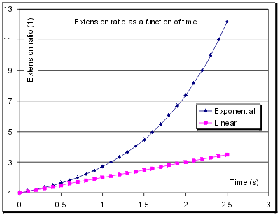
In T-SIM(B-SIM) material graphs the exponential deformation history is used to calculate stresses. Seven "epsilons" (e, strain rates) from 0.01 to 100 1/s are used to calculate seven stress/strain curves.
The curves are generated in the following way:
This algorithm describes how the stress-strain curves are calculated. It is obvious that if the deformation history is different, the generated stress-strain curves are also different.
The point 3) is quite complicated to describe. To get the stress, an integral is numerically calculated from time 0 to time t using small steps in time to get an exact result. During the integration it MUST be known how the l is changing in the time range from 0 to t. This is the reason why the function l(t) MUST be exactly known. The easiest way to assure it is to use one of the deformation histories described above.
Supposing the data were measured using on of the described ways, T-SIMFIT can be used to fit the stress-strain curves and export the T-SIM /B-SIM material file.
Run T-SIMFIT and click on View / Test & material data to enter information necessary to fit the measured data correctly:
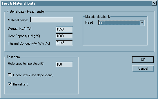
In Material data - Heat transfer specify material name, its density, heat capacity and thermal conductivity. Use material databank to load the data for typical polymers.
In Test data specify the reference temperature (usually,
the reference temperature is the lowest measured one).
Select also the test type - check Linear strain-time dependency if
l(t) is a linear function of time. Do not check if the l(t)
is an exponential function of time.
Check Biaxial test if the tests performed were equibiaxial. Do not check
if the tests were uniaxial.
Once everything is specified, click OK to confirm the changes.
Now, in the document view, specify the sample temperature, length, thickness and width. You do not have to enter the length, thickness and width. However, if the strain-time dependency is linear, the sample length must be specified.
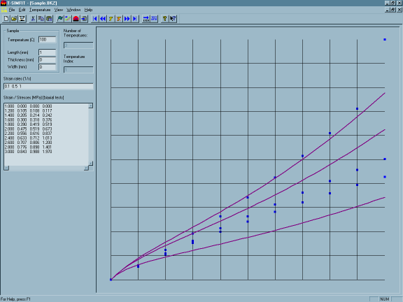
In Strain rates, specify all the used strain rates at the specified temperature (in this case 0.1, 0.5 and 1.0 1/s).
In Strain / Stresses enter on each row the extension ratio l and the measured stresses s at all used strain rates. In this case, one number (l) is followed by there values of stress for strain rate 0.1, 0.5 and 1.0 1/s.
Click on Temperature / Add to add a new temperature and enter additional stress-strain curves.
Repeat the procedure describe above until all the measured data are specified. Then click on File / Save to save the data.
Once the stress-strain data are entered into T-SIMFIT, the fitting procedure can be initialized. Click on File / Fit the data to display the following dialog:
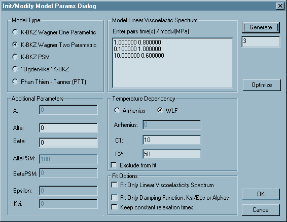
This dialog enable to select the model type for the fit, to enter the initial guess of parameters, to set some fitting options and to "optimize" the fitted spectrum.
Model type
For almost all materials any type of K-BKZ model can be used, exclusive
the "Ogden-like" K-BKZ, because this model is not supported in T-SIM
/ B-SIM.
PTT at this moment is not included in T-SIM / B-SIM (versions 4.15 /
2.15).
For strain-hardening materials, use K-BKZ Wagner Two Parametric.
Additional parameters and Linear
viscoelastic spectrum
Usually you do not have to take care about these values - just click
on Generate and an initial set of the model parameters will be generated
automatically. Below the Generate button there is an edit box where
you can specify the number of time / modul parameters before clicking
on Generate.
Temperature dependency
From T-SIM V4.0 and B-SIM V2.0, only WLF is supported. Select WLF.
A fit with Arrhenius will be exported into T-SIM / B-SIM material file
with default WLF parameters (C1=17.44, C2=51.6).
You can check Exclude from fit to exclude the temperature dependency
from fit. If you do so, the temperature dependency parameters will keep
their values constant during the fitting procedure.
Fit options
Fit options normally need not be used, but they can help if the fit
with the default settings is not possible.
Optimize button - use it when you want to generate an uniform relaxation times distribution. The following window appears when you click on Optimize:
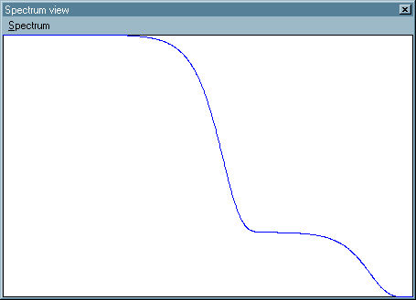
The blue curve represents the linear viscoelastic spectrum
(values on x and y axis are time and relax. modul).
Now click on Spectrum / Optimize and wait until the following dialog
is displayed:
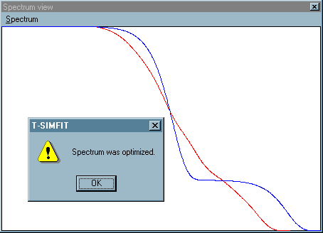
The red curve corresponds to the "optimized" spectrum which can look like this:
Time Modul
0.001000 0.126341
0.010000 0.000000
0.100000 0.024217
1.000000 0.063886
10.000000 0.027348
100.000000 0.012250
1000.000000 0.031387
Click OK to close the Spectrum view and start the fitting procedure to fit the measured data using spectrum with seven time / modul pairs.
Click on OK in Init model parameters dialog. The fit starts displaying a window with question: "Run the calculation ?" Click Yes to run, No or Cancel to get back to Init model parameters dialog.
The following dialog appears when you select Yes:

It informs about the fit progress. The title bar indicates number of iterations.
Check Cancel after this iteration step if you want to stop the fitting (for example when you see the fitting curves are close enough to the measured points, but the calculation is still running). The calculation will stop after the current iteration. The values of the used model parameters will be saved.
Check Pause after this iteration step to modify model params if you want to pause the fitting procedure. The calculation will pause after the current iteration. Init / Modify Model Params dialog will appear and you can change model type, type of temperature dependency and modify all model parameters. Click OK to update model parameters. Click Cancel and parameters will remain unchanged. In both cases the calculation continues.
Click Cancel Now if you want to stop the fitting immediately. The calculation stops immediately and values of the used model parameters are lost.
Once the fit is done, click on File / Save to save the fitted parameters. Click also on File / Save to T-SIM to save the fitted model into T-SIM / B-SIM material file.